Transformer vs. LSTM for Time Series Forecasting

This article provides a comprehensive guide to building, training, and comparing Long Short-Term Memory (LSTM) and Transformer models for next-day univariate time series forecasting. Utilizing real-world public transit data, we will cover:

• Structuring and windowing time series data for supervised learning.
• Implementing concise LSTM and Transformer architectures in PyTorch.
• Evaluating and comparing model performance using Mean Absolute Error (MAE) and Root Mean Squared Error (RMSE) on held-out test data.

Let's begin.

Introduction

Time series data, from daily weather patterns to stock market fluctuations, is ubiquitous. For complex time series datasets, advanced models like ensemble methods or deep learning architectures often prove more effective than traditional forecasting techniques. This article demonstrates the training and application of two prominent deep learning architectures—Long Short-Term Memory (LSTM) networks and Transformers—for time series data. Beyond simply utilizing these models, the goal is to explore their fundamental differences in handling temporal data and assess if one offers a distinct performance advantage. A basic understanding of Python and machine learning principles is recommended.

Problem Setup and Data Preparation

For this comparative analysis, we focus on a univariate time series forecasting task: predicting the (N+1)th value given the preceding N time steps. Our chosen dataset is the publicly available Chicago rides dataset, which provides daily bus and rail passenger counts from the Chicago public transit network, dating back to 2001.

The initial step involves importing necessary libraries—pandas, NumPy, Matplotlib, and PyTorch for data manipulation and model building, alongside scikit-learn for evaluation metrics—and loading the dataset.

import pandas as pd
import numpy as np
import matplotlib.pyplot as plt

import torch
import torch.nn as nn
from sklearn.metrics import mean_squared_error, mean_absolute_error

url = "https://data.cityofchicago.org/api/views/6iiy-9s97/rows.csv?accessType=DOWNLOAD"
df = pd.read_csv(url, parse_dates=["service_date"])
print(df.head())

To mitigate the impact of post-COVID data, which significantly alters passenger distribution and could skew predictive power, we filter the dataset to include records only up to December 31, 2019.

df_filtered = df[df['service_date'] <= '2019-12-31']

print("Filtered DataFrame head:")
display(df_filtered.head())

print("
Shape of the filtered DataFrame:", df_filtered.shape)
df = df_filtered

A visualization of the filtered time series data is shown below:

df.sort_values("service_date", inplace=True)
ts = df.set_index("service_date")["total_rides"].fillna(0)

plt.plot(ts)
plt.title("CTA Daily Total Rides")
plt.show()

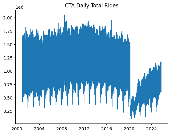CTA Daily Total Rides Time Series Data (pre-2020)

The time series data is then partitioned into training and test sets. Crucially, for time series forecasting, this split must be sequential, not random, ensuring that all training data precedes the test data chronologically. The following code allocates the first 80% of the time series for training and the subsequent 20% for testing.

n = len(ts)
train = ts[:int(0.8*n)]
test = ts[int(0.8*n):]

train_vals = train.values.astype(float)
test_vals = test.values.astype(float)

Raw time series data requires transformation into labeled sequences (X, y) with a fixed time window for neural network training. For instance, with a 30-day window, the input (X) would comprise the first 30 days, and the output (y) would be the 31st day's value. This method prepares the dataset for supervised learning while preserving its inherent temporal integrity.

def create_sequences(data, seq_len=30):
    X, y = [], []
    for i in range(len(data)-seq_len):
        X.append(data[i:i+seq_len])
        y.append(data[i+seq_len])
    return np.array(X), np.array(y)

SEQ_LEN = 30
X_train, y_train = create_sequences(train_vals, SEQ_LEN)
X_test, y_test = create_sequences(test_vals, SEQ_LEN)

# Convert our formatted data into PyTorch tensors
X_train = torch.tensor(X_train).float().unsqueeze(-1)
y_train = torch.tensor(y_train).float().unsqueeze(-1)
X_test = torch.tensor(X_test).float().unsqueeze(-1)
y_test = torch.tensor(y_test).float().unsqueeze(-1)

With the data prepared, we are now ready to proceed with training, evaluating, and comparing our LSTM and Transformer models.

Model Training

PyTorch will be used for the modeling phase, offering the essential classes required to define both recurrent LSTM layers and encoder-only Transformer layers, which are ideal for predictive tasks.

The LSTM-based Recurrent Neural Network (RNN) architecture is defined as follows:

class LSTMModel(nn.Module):
    def __init__(self, hidden=32):
        super().__init__()
        self.lstm = nn.LSTM(1, hidden, batch_first=True)
        self.fc = nn.Linear(hidden, 1)

    def forward(self, x):
        out, _ = self.lstm(x)
        return self.fc(out[:, -1])

lstm_model = LSTMModel()

For next-day time series forecasting, the encoder-only Transformer architecture is implemented as:

class SimpleTransformer(nn.Module):
    def __init__(self, d_model=32, nhead=4):
        super().__init__()
        self.embed = nn.Linear(1, d_model)
        enc_layer = nn.TransformerEncoderLayer(d_model=d_model, nhead=nhead, batch_first=True)
        self.transformer = nn.TransformerEncoder(enc_layer, num_layers=1)
        self.fc = nn.Linear(d_model, 1)

    def forward(self, x):
        x = self.embed(x)
        x = self.transformer(x)
        return self.fc(x[:, -1])

transformer_model = SimpleTransformer()

In both architectures, the final layer maintains a consistent structure: its input corresponds to the hidden representation dimensionality (32 in this example), and a single neuron is utilized to output a univariate forecast for the next day's total rides.

Next, we proceed to train both models and evaluate their performance using the designated test data.

def train(model, X, y, epochs=10):
    model.train()
    opt = torch.optim.Adam(model.parameters(), lr=1e-3)
    loss_fn = nn.MSELoss()

    for epoch in range(epochs):
        opt.zero_grad()
        out = model(X)
        loss = loss_fn(out, y)
        loss.backward()
        opt.step()
    return model

lstm_model = train(lstm_model, X_train, y_train)
transformer_model = train(transformer_model, X_train, y_train)

To assess the performance of the models in this univariate time series forecasting task, we will utilize two widely accepted metrics: Mean Absolute Error (MAE) and Root Mean Squared Error (RMSE).

lstm_model.eval()
transformer_model.eval()

pred_lstm = lstm_model(X_test).detach().numpy().flatten()
pred_trans = transformer_model(X_test).detach().numpy().flatten()
true_vals = y_test.numpy().flatten()

rmse_lstm = np.sqrt(mean_squared_error(true_vals, pred_lstm))
mae_lstm  = mean_absolute_error(true_vals, pred_lstm)

rmse_trans = np.sqrt(mean_squared_error(true_vals, pred_trans))
mae_trans  = mean_absolute_error(true_vals, pred_trans)

print(f"LSTM RMSE={rmse_lstm:.1f}, MAE={mae_lstm:.1f}")
print(f"Trans RMSE={rmse_trans:.1f}, MAE={mae_trans:.1f}")

Results Discussion

Below are the performance metrics obtained from our models:

LSTM RMSE=1350000.8, MAE=1297517.9 Trans RMSE=1349997.3, MAE=1297514.1

The results demonstrate remarkable similarity between the two models, making it challenging to definitively declare one superior. While the Transformer shows a marginally better performance, the difference is negligible. This similarity likely stems from the nature of the univariate time series data used; its reasonably consistent patterns allow both architectures, despite their intentionally minimal complexity, to effectively solve the forecasting problem. Readers are encouraged to re-run the process without filtering post-COVID data, maintaining the 80/20 training/testing split, to investigate if the performance disparity between the models becomes more pronounced.

Furthermore, the short-term nature of this forecasting task—predicting only the next-day value—contributes to the similar outcomes. A more complex task, such as predicting values 30 days into the future, would likely amplify the differences in error rates between the models, potentially showing the Transformer outperforming the LSTM, though this is not a universal guarantee.

Conclusion

This article successfully demonstrated how to approach a time series forecasting task using two distinct deep learning architectures: LSTM and the Transformer. We covered the complete workflow, from data acquisition and preparation to model training, evaluation, comparison, and interpretation of the results.